目标检测新范式:End-to-End Object Detection with Transformers
| 标题 | Keep your Eyes on the Lane: Real-time Attention-guided Lane Detection |
|---|---|
| 年份: | 2020 年 5 月 |
| GB/T 7714: | [1] Carion N , Massa F , Synnaeve G , et al. End-to-End Object Detection with Transformers[J]. 2020. |
| DETR是FIR提出的基于Transformers的端到端目标检测,没有NMS后处理步骤、没有anchor,结果在coco数据集上效果与Faster RCNN相当,且可以很容易地将DETR迁移到其他任务例如全景分割。 |
原文链接:【论文笔记】从Transformer到DETR (zhihu.com)
1 Transformer原理
1.1 Transformer的整体架构
Transformer是2017年NIPS上的文章,题目为Attention is All You Need。它使用attention组成了encoder-decoder的框架,并将其用于机器翻译。它的大致结构如下:

每个句子先经过六个Encoder进行编码,然后经过六个Decoder进行解码,得到最后的输出
![]()
1.2 Transformer Encoder
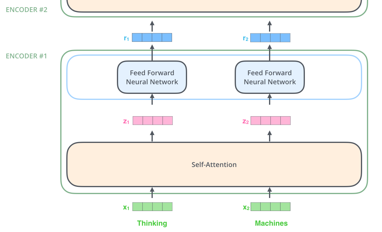
如上图所示,Encoder的输入是词向量(大概是word2vec之类的编码)和Positional Encoding(二者相加之后送入第一个Encoder),然后经过Self Attention和Layer Norm,最后是一个Feed Forward Network。另外每个Encoder中还有两个Skip Connection。这种Encoder结构重复六次之后就得到了句子的编码。我会在接下来几个subsection中介绍Encoder中的各个function。
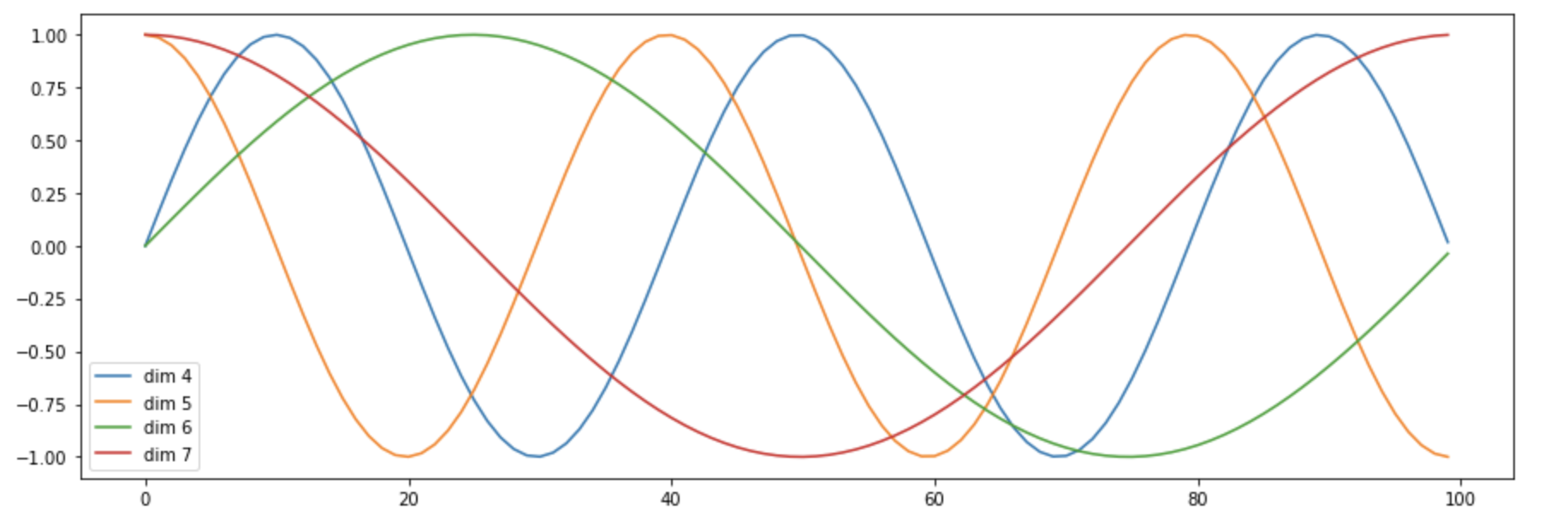
1.2.1 Positional Encoding
Positional Encoding旨在为每个特征的位置与通道进行编码,其公式如下所示: $$ PE_{(pos,2i)} = sin(pos/100^{2i/d_{model}}) $$
$$ PE_{(pos,2i+1)} = cos(pos/1000^{2i/d_{model}}) $$
其中i是通道的下标,pos是位置的下标,$d_{model}$是特征的总通道数。
奇数位置的PE使用余弦来表示,偶数位置的PE使用正弦表示。 $1000^{2i/d_{model}}$ 用于控制不同通道PE的波长(这样不同通道的特征有一定的区分性)。
PE最后与输入的特征相加,并被送到第一个Encoder中(有种CoordConv的感觉)。
这篇文章可视化了Positional Encoding的前几维,大概是下图这样:
1.2.2 Self Attention
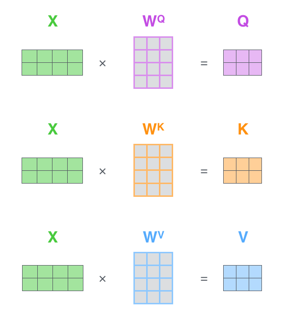
Encoder中的第一个模块是Self Attention,它可以用以下公式来表示 $$ \operatorname{Attention}(Q, K, V)=\operatorname{softmax}\left(\frac{Q K^{T}}{\sqrt{d_{k}}}\right) V $$ 如下图:
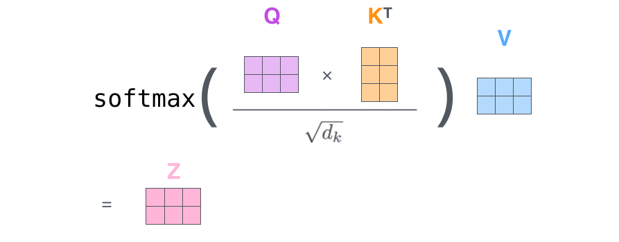
其中$d_k$是特征的维度,Q、K、V分别是Query、Key、Value,是对X分别进行三次矩阵乘法得到的向量:
作者在文中采用了多头(Multi-Head)Attention,就是h个Self Attention的结果Cat起来,然后压到一个较低的维度。
1.2.3 Feed Forward Network(FFN)
Encoder最后的操作是带Skip Connection的FFN。其本质是FC-ReLU-FC的操作。 $$ \operatorname{FFN}(x)=\max \left(0, x W_{1}+b_{1}\right) W_{2}+b_{2} $$
1.3 Transformer Decoder
Decoder的第一个Attention与Encoder类似,只不过是带了一个与位置有关的Mask(预测第i个位置的时候,输入是前i-1个位置的embedding,后面位置的编码被Mask掉了)。
第二个Attention依然是同样的结构,区别在其输入不同:Q来自于Decoder,K和V来自于Encoder。这种做法大抵是为了结合Encoder和Decoder的信息。
FFN的结构也与Encoder类似。
最后在经过6个Decoder之后,由线性层和SoftMax得到每一个单词的翻译结果。
2 DETR的原理
看代码后发现它的输出是定长的:100个检测框和类别。某自动化所的学长说,这种操作可能跟COCO评测的时候取top 100的框有关,我认为他说的有道理。
从这种角度看,DETR可以被认为具有100个adaptive anchor,其中Encoder和Object Query分别对特征和Anchor进行编码,最后用Decoder+FFN得到检测框和类别。
这篇文章也从侧面说明100个Anchor完全够用。但是进一步想,100个Anchor其实也是有一些冗余输出的:很多图里面物体很少,并不能用完100个检测框吧。
这一点在篇车道线检测的paper中也有体现,他设置的N为5可以达到最优效果
2.1 DETR的结构
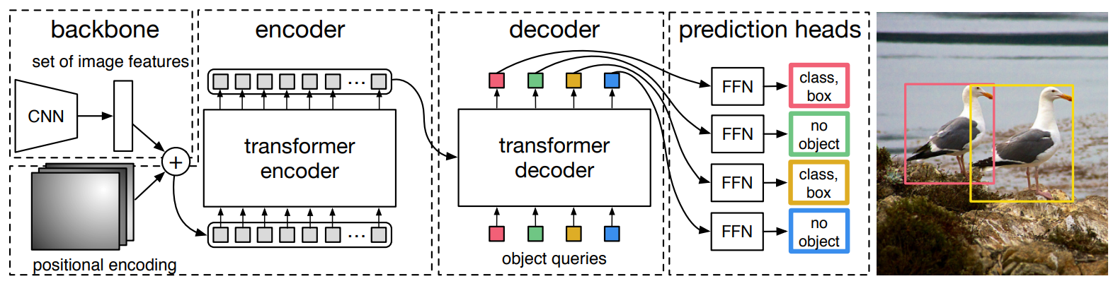
DETR的整体结构Transformer类似:Backbone得到的特征铺平,加上Position信息之后送到一坨Encoder里,得到一些candidates的特征。这100个candidates是被Decoder并行解码的(需要很大的显存,但实现的时候可写成不并行的),以得到最后的检测框。
2.2 DETR Encoder
网络一开始是使用Backbone(比如ResNet)提取一些feature,然后降维到$d×HW$。
Feature降维之后与Spatial Positional Encoding相加,然后被送到Encoder里。
为了体现图像在x和y维度上的信息,作者的代码里分别计算了两个维度的Positional Encoding,然后Cat到一起。
pos_x = torch.stack((pos_x[:, :, :, 0::2].sin(), pos_x[:, :, :, 1::2].cos()), dim=4).flatten(3)
pos_y = torch.stack((pos_y[:, :, :, 0::2].sin(), pos_y[:, :, :, 1::2].cos()), dim=4).flatten(3)
pos = torch.cat((pos_y, pos_x), dim=3).permute(0, 3, 1, 2)
FFN、LN等操作也与Transformer类似。Encoder最后得到的结果是对N个物体编码后的特征。
2.3 DETR Decoder
DETR Decoder的结构也与Transformer类似,区别在于Decoder并行解码N个object。
每个Decoder有两个输入:一路是Object Query(或者是上一个Decoder的输出),另一路是Encoder的结果。
我一开始不明白Object Query是怎样得到的。后来从代码看,Object Query是一组nn.Embedding的weight(就是一组学到的参数)。
另外一个与Transformer不同的地方是,DETR的Decoder也加了Positional Encoding。
最后一个Decoder后面接了两个FFN,分别预测检测框及其类别。
2.4 Bipartite Matching
由于输出物体的顺序不一定与ground truth的序列相同,作者使用二元匹配将GT框与预测框进行匹配。其匹配策略如下:
最后的损失函数:
2.5 Experiment and Ablation
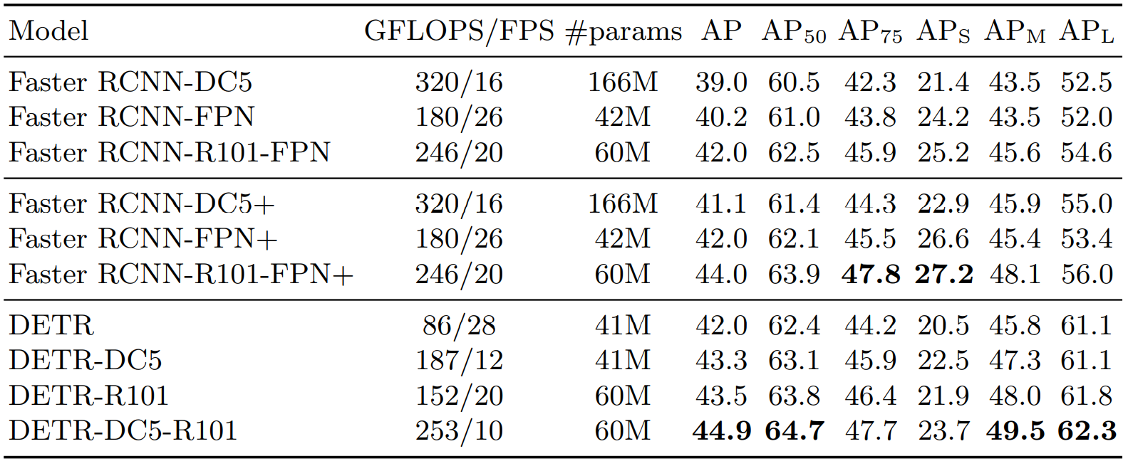
2.5.1 性能对比
与Faster RCNN有可比性,小目标要差一些
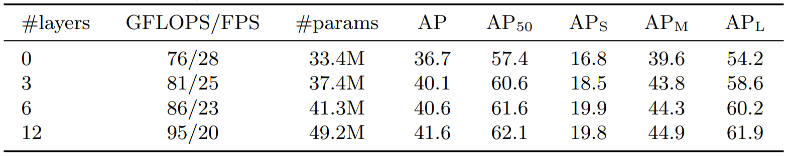
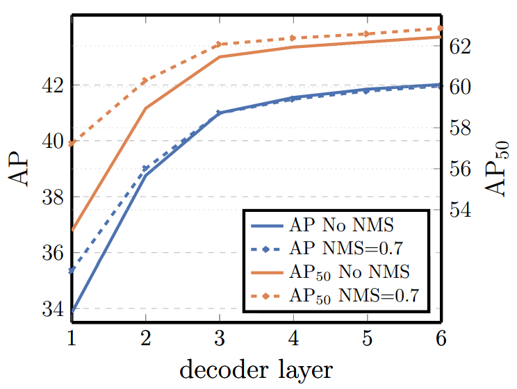
2.5.2 测试Encoder和Decoder要用多少层
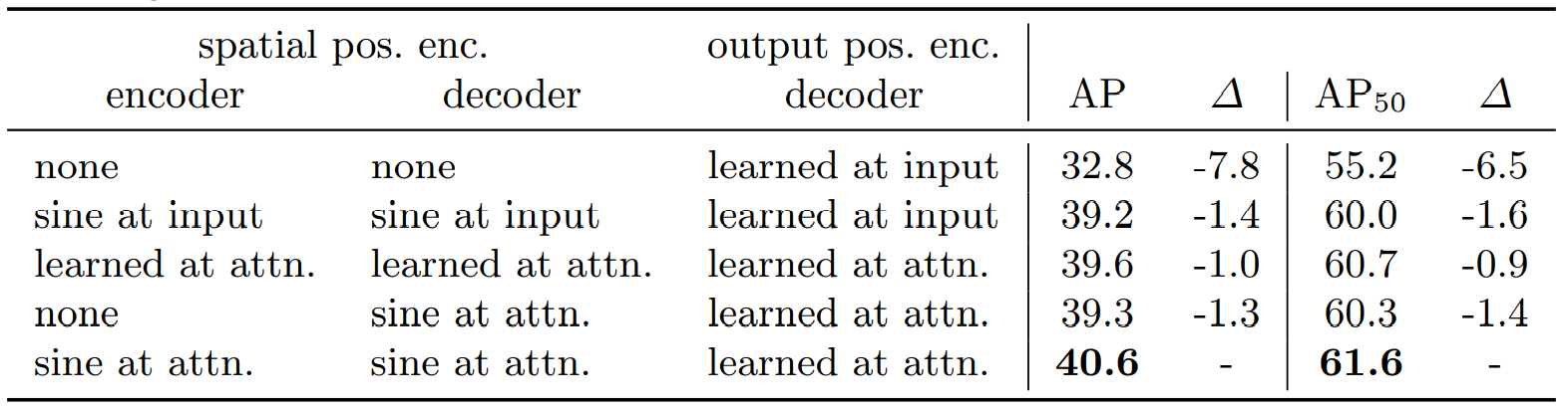
2.5.3 测试不同的Positional Encoding
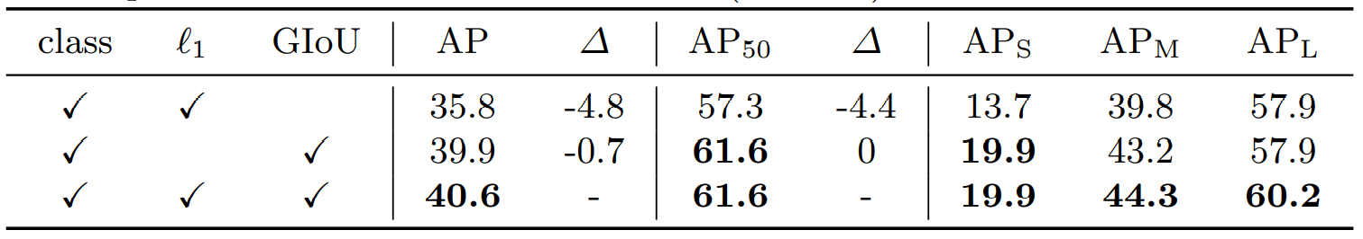
2.5.4 测试Loss
参考资料
【论文笔记】从Transformer到DETR (zhihu.com)
The Illustrated Transformer – Jay Alammar – Visualizing machine learning one concept at a time.
End-to-End Object Detection with Transformers_feng__shuai的博客
项目地址:https://github.com/facebookresearch/detr
快速查看detr效果:https://github.com/plotly/dash-detr